KWDB SQL Compilation and Optimization

1. Overview

KWDB is a distributed multi-model database product designed for AIoT scenarios. It supports establishing both time-series and relational databases within the same instance and performing fused processing of multi-model data. KWDB possesses efficient time-series data processing capabilities such as millions of device access, millions of data writes per second, and billions of data reads per second. It also features stability, security, high availability, and easy operation and maintenance.

KWDB's SQL engine consists of a parser, optimizer, and executor. The compilation and optimization section mainly introduces the parser and optimizer.

The main function of the parser is to convert user-input SQL statements into structures that KWDB can execute, while performing necessary syntax validation. It mainly includes three steps: lexical analysis, syntax analysis, and semantic analysis.

The main function of the optimizer is to perform structural equivalence transformations on the structures generated by the parser using rule-based and cost-based optimization, making them more efficient and lower-cost without changing the original meaning of the SQL. It mainly includes RBO optimization, CBO optimization, and multi-model computation optimization.

2 KWDB Query Compilation and Optimization Architecture

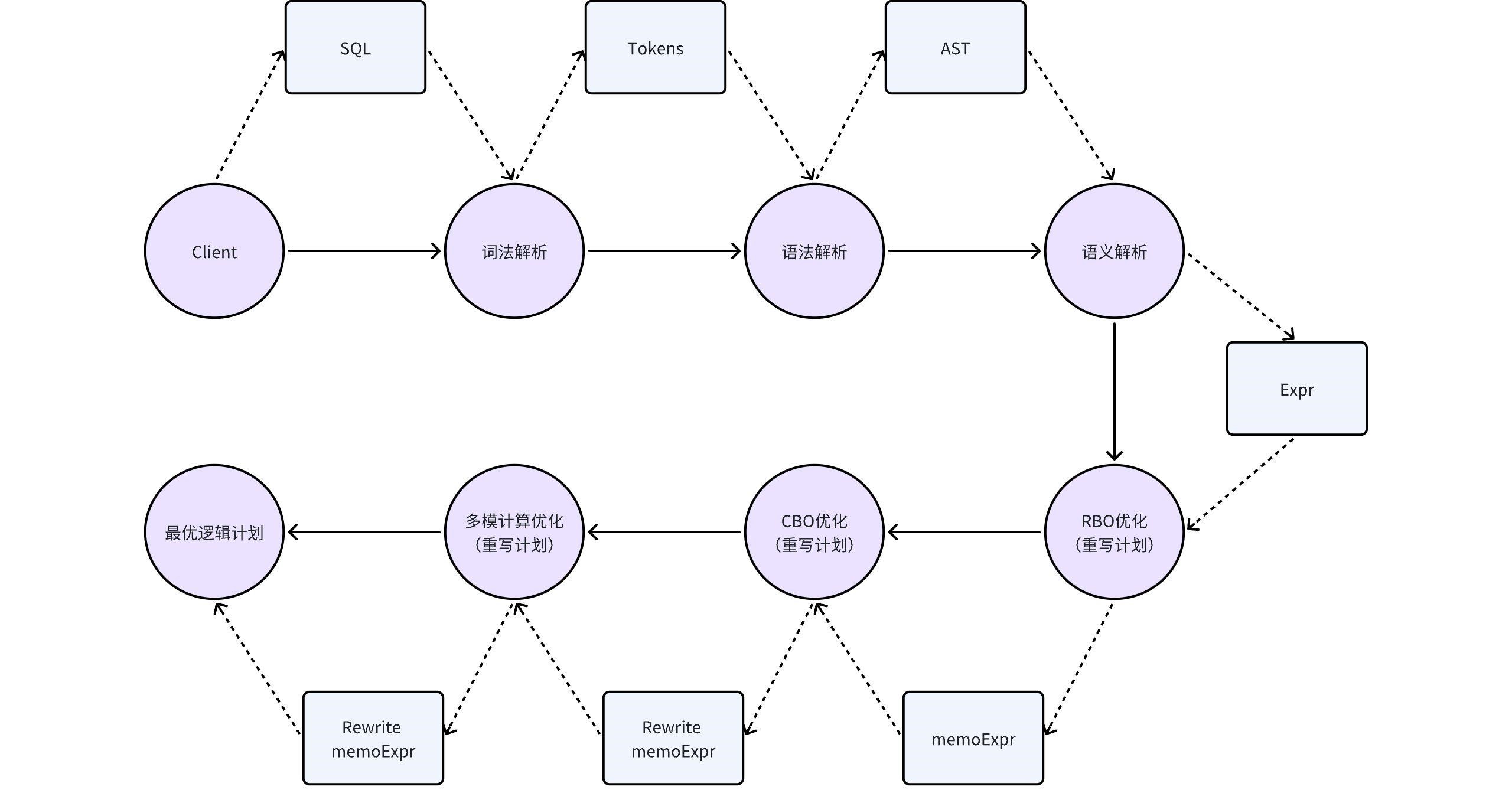
During the compilation phase, KWDB performs three main steps on SQL statements: lexical analysis, syntax analysis, and semantic analysis. During the semantic analysis phase, KWDB also performs RBO optimization on the plan to make it better.

2.1 Lexical Analysis

KWDB's lexical analysis converts SQL statements from a character stream into a list of lexical tokens (such as keywords, identifiers, constants, and operators) based on the lexical units defined in the yacc file.

The specific steps are as follows:

• Remove comments and whitespace.
• Recognize lexical units: scan the SQL character stream to decompose and identify lexical units.
• Build tokens: arrange the identified lexical units in SQL order to form a list.

For example, with the following query statement:

SELECT a, b FROM t WHERE c > 30;

The result of lexical analysis is as follows:

SELECT (keyword)
a (identifier)
, (separator)
b (identifier)
FROM (keyword)
t (identifier)
WHERE (keyword)
c (identifier)
> (operator)
30 (constant)
; (separator)

2.2 Syntax Analysis

KWDB's syntax analysis traverses the tokens for recognition based on the grammar defined in the yacc file, determining whether there are syntax errors and specification conflicts.

The cases where an abstract syntax tree (AST) cannot be generated are as follows:

• Syntax error: validation fails when determining that reduction (generating syntax) is needed, such as undefined syntax.
• Shift-reduce conflict: unable to decide whether to shift (continue reading tokens) or reduce (generate syntax), usually because the symbols in the input string may match the right sides of multiple productions.
• Reduce-reduce conflict: multiple reduction operations are possible, unable to determine which reduction rule to use, indicating ambiguity.

After each reduction is completed correctly until the token traversal ends, an abstract syntax tree (AST) is ultimately generated.

2.3 Semantic Analysis

KWDB's semantic analysis performs in-depth analysis on the AST of the query to ensure that the query is logically and semantically valid and can be executed correctly.

The specific operations are as follows:

• Check whether the query is a valid statement in SQL language, including checks for table and column existence, data type validation, permission checks, and constraint validation.
• Resolve names, such as table names or variable name values.
• Eliminate intermediate operations, such as replacing 0.5+0.5 with 1.0. This is also known as constant folding.
• Determine the data type for intermediate results, such as when the query statement contains a subquery.

After this step, the generated plan can already be converted into an execution plan, but this plan is not the optimal plan. Subsequent optimization is still required.

2.3 RBO Optimization

RBO (rule-based optimization) is rule-based optimization. The principle is equivalent to relational algebra equivalence transformation, replacing the original expression with a more efficient equivalent expression. Typical rules include column pruning, predicate pushdown, projection elimination, and so on.

The detailed analysis is as follows:

• Column Pruning

  Suppose table t has four columns: a, b, c, d. Given the following query statement:

  SELECT a FROM t WHERE b > 5;

  This query can either read all data from table t, then filter according to the conditions, then project, and finally get the data of column (a). Alternatively, column pruning can be performed first, reading only columns a and b, then filtering according to the filter conditions, and finally outputting the data. Column pruning can avoid consuming some unnecessary resources.

• Min-Max Elimination

  Given the following query statement:

  SELECT min(a) FROM t;

  This statement can be transformed into:

  SELECT a FROM t ORDER BY a DESC LIMIT 1; 

  This query method is more efficient than performing aggregation.

• Projection Elimination

  Suppose both tables t and tt have four columns: a, b, c, d.

  Given the following query statement:

  SELECT t1.a t2.b FROM t AS t1 JOIN (SELECT a, b, c FROM tt) AS t2 ON t1.a=t2.a;

  This query statement's projection columns only need column a from table t and column b from table tt. However, the projection columns of the subquery on the right side of the join contain three columns: a, b, and c. Column c is not needed in the outer layer, so column c will be eliminated in the plan.

• Predicate Pushdown

  Given the following query statement:

  SELECT * FROM t, tt WHERE t.a > 3 AND tt.b < 5;

  Assuming both t and tt have 100 rows of data, if we first perform a Cartesian product of t and tt and then filter, we need to process 10,000 rows of data. If we can perform predicate condition filtering first (pushing down the filter conditions of each table into the select calculation), the data volume may be greatly reduced. For example, there are 10 rows of data in table t that meet the condition t.a > 3, and 8 rows of data in table tt that meet the condition tt.b < 5. After filtering first, performing the Cartesian product only requires processing 80 rows.

  Predicate pushdown means placing filter conditions as close to the leaf nodes as possible.

Plans optimized through RBO have higher performance efficiency, better performance, and lower costs than unoptimized plans.

This concludes the introduction to RBO optimization. KWDB also performs more in-depth CBO optimization and multi-model scenario computation optimization on SQL. Please refer to Sections 3 and 4.

3 Optimization for Multi-Model Computation

3.1 KWDB Multi-Model Computation Localization

3.1.1 Computation Localization Concept

Query is executed within the time-series engine as much as possible, which reduces data transmission and allows data to be processed locally, improving query efficiency. This process of finding the maximum plan tree supported by the time-series engine is called computation localization.

3.1.2 Basic Approach for Computation Localization

Query statements are parsed by the syntax parser into a tree-structured expression. Each layer of expression is subsequently converted into corresponding operators executed by the execution engine. This tree structure is called a memo tree. During the construction of the memo tree, some scalar expressions need to be evaluated and processed, such as filters. After the memo tree is basically constructed, it needs to be traversed from top to bottom to find the maximum tree that can be computed locally in the time-series engine.

3.1.3 Processing for Computation Localization at Each Layer

1. For the scan layer

   • All time-series scans execute computation localization in the time-series engine

2. For the filter layer

   • Need to decompose the filter expression to determine which filter conditions can achieve computation localization and which filter conditions cannot achieve computation localization, and record them
   • Perform a series of operations on the recorded results to obtain the final set of filters that need computation localization
   • The part that can achieve computation localization is placed as a filter operator in the time-series engine for execution
   • The relational engine rebuilds a new filter layer based on the part that cannot achieve computation localization
   • The relational engine receives the data processed by the time-series filter and performs further filtering

   This completes the computation localization processing for the filter layer.

3. For the group layer

   GroupBy, ScalarGroupBy, and Distinct logic are consistent. First, let's explain these three terms:

   • GroupBy: query has aggregate functions and has group by
   • ScalarGroupBy: query only has aggregate functions, without group by
   • DistinctOnExpr: query only has group by, without aggregate functions

   The local computation of the group layer needs to determine whether the following two locations can achieve computation localization:

   • group by: check whether group by columns can achieve computation localization
   • aggregation: check whether aggregate functions, aggregate function inputs (including types, count, etc.), and aggregate function operations can achieve computation localization

   Special notes:

   • For ScalarGroupBy layer, condition 1 does not need to be checked
   • For DistinctOnExpr layer, condition 2 does not need to be checked
   • This layer cannot be split; if one location cannot be computed locally, the group by layer cannot be computed locally

4. For the projection layer

   • When processing projection, check whether this layer's projection operations can achieve computation localization
   • For example, if projection columns contain int + float, it is not supported by the time-series engine
   • As long as there is a situation where computation localization cannot be performed, this layer will not perform computation localization

5. For the limit layer

   • The limit layer can use computation localization processing in the time-series engine
   • With multiple nodes, the gateway node needs to perform secondary limit aggregation on the results

6. Other layers

   • Other operators are not yet implemented, such as join expressions are not yet supported for computation localization in the time-series engine
   • Will be gradually supported in subsequent versions

3.1.4 Computation Localization Control

We hope to have a flexible, adjustable mechanism to control the computation localization judgment for each layer. Below is an introduction to a mechanism for controlling computation localization: the Computation Localization Whitelist.

3.1.4.1 Computation Localization Whitelist

The computation localization whitelist is a system table used to control whether expressions can be computed locally. It records all expressions supported by the time-series engine. The whitelist contains the following elements:

• Locally Executable Operations: indicates whether the operator of this expression can be computed locally in the time-series engine
• Parameter Count: indicates the number of parameters for this expression
• Parameter Type: indicates the parameter types for this expression, can represent multiple parameter types, is an array
• Locally Computable Position: indicates where this expression appears in the query
• Default Enable: whether computation localization is enabled by default, can be manually changed
• Supported Types: supports expression types, such as const, column, agg, binary, compare

Below is an example of a whitelist:

Locally Computable Operator or Function	Parameter Count	Parameter Type	Locally Computable Position	Default Enable	Supported Types
+	2	int;int	where	true	Constant; Column Type

In this example, the whitelist allows "+" operator expressions that meet the following conditions to be computed locally:

1. The parameter count of the "+" operator is 2, i.e., left and right parameters
2. The parameter types of the "+" operator are: left parameter type is int, right parameter type is int
3. The "+" operator appears in the where condition
4. The result of the "+" operator is a constant or column type

3.1.4.2 Using Whitelist to Control Computation Localization

Below is an introduction to how to determine if an expression is in the whitelist.

1. Each row in the whitelist represents an expression that can be computed locally. Perform hash encoding (hash code) based on the expression's operator (or function) name, parameter count, and parameter types.
2. Use this hash encoding as the key, and the allowed positions and expression's output type as the value, put them into a map.
3. When checking whether an expression at a certain layer can be computed locally, first perform hash encoding based on the expression's operator, parameter count, and parameter types to get a hash code. Use this hash code to retrieve the value from the map.
4. If a value can be retrieved, verify whether the allowed positions and the expression's output type can be computed locally. This information is stored in the value of the map.
5. Following the above steps to check the expression. If the conditions are met, it means the whitelist allows this expression to be computed locally.

3.1.5 Example Illustration of Computation Localization Judgment

Below is an example to introduce the process of judging computation localization.

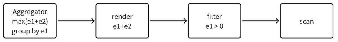
Given the query select max(e1+e2) from d1.t1 where e1 > 0 group by e1; where column e1 is of type int and column e2 is of type float.

Assume our whitelist is as follows:

Locally Computable Operator or Function	Parameter Count	Parameter Type	Locally Computable Position	Default Enable	Supported Types
max	1	int	Projection Column	true	Constant; Column Type
+	2	int;float	All Positions	true	All Types (including Const, Column, Binary, Compare, Agg)
>	2	int;int	where	true	All Types

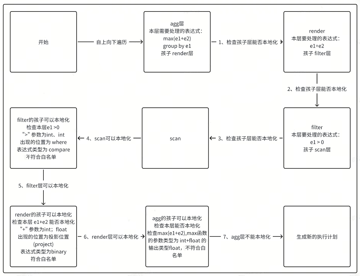
First, the memo tree generated by this query is as follows.

The following figure shows the computation localization process for this memo tree.

3.1.6 Main Logic Entry for Computation Localization

1. CheckWhiteListAndAddSynchronize: Entry point for computation localization logic
2. CheckWhiteListAndAddSynchronizeImp: Main body of computation localization logic, checks whether each layer's operators can be computed locally, including checking functions for each layer
3. CheckExprCanExecInTSEngine: Determines whether this layer's expression can be computed locally by the time-series engine
4. SetAddSynchronizer: Adds concurrency flag to this layer

Operators using time-series localization support concurrency. Therefore, after finding the maximum tree that can be computed locally, a concurrency flag is added so that the time-series engine can execute concurrently.

3.2 Statistics and CBO

The query optimizer uses a cost-based optimizer, which uses statistics to evaluate the expected costs of different query plans and selects the execution plan with the lowest cost. The main flow of query optimization is shown in the figure:

3.2.1 Statistics

Statistics serve as the data source for the query optimizer. The statistics collection process is shown in the figure:

• TableReader: Table reader, reads table data.
• TsSampler: Sampler, collects table-level statistics, as well as samples and cardinalities for input columns.
• SampleAggregator: Sampling aggregator, aggregates results from multiple samplers and persists the statistics.

3.2.2 Cost Model

The cost model consists of cost calculation formula functions for different operation types. Its main behaviors in the optimizer include:

• For incoming candidate expressions, based on the statistics in the logical expression tree, estimate the actual execution cost.
• Distribute the estimated cost to the corresponding expressions. If the candidate expression's cost is lower than any other expression in the memo, it will become the best new expression for that group.

In Costor.go, with ComputeCost as the main function entry, it calls corresponding objects and their functions to estimate the execution cost of expressions.

3.2.3 Plan Enumeration

• The query optimizer uses the Cascades framework, optimizing from top to bottom
• In the initial CBO phase, the AST is transformed into a normalized plan
• Plan enumeration enumerates all expressions equivalent to the normalized plan in sequence and estimates the cost of each expression
• Finally, the plan with the minimum estimated cost is output, which is the optimal plan

The following provides an example:

3.3 Summary

This article provides an overview of KWDB's macro process in query optimization and compilation, as well as the extensions and optimizations made in conjunction with the multi-model engine. The KWDB project itself is still iterating rapidly. Everyone is welcome to visit the KWDB code repository to learn about the latest features and innovations in this field.