KWDB SQL Execution

1. Overview

KWDB is a distributed multi-model database product designed for AIoT scenarios. It supports establishing both time-series and relational databases within the same instance and processing multi-model data in a fused manner. KWDB provides efficient time-series data processing capabilities such as millions of device connections, millions of data writes per second, and billions of data reads per second. It features stability, security, high availability, and easy operation and maintenance.

KWDB's SQL engine consists of a parser, optimizer, and executor. This issue of KWDB SQL execution content primarily introduces the executor.

KWDB's distributed executor distributes plan fragments from each node to the corresponding nodes, where each node processes data based on the received plan fragments. The advantages of distributed execution are: first, it utilizes the characteristics of distributed multiple nodes, where each node implements parallel computation to accelerate calculation; second, distributed execution performs computation at the nodes where the data source is located, implementing "in-place computation," which reduces data network transmission.

2. KWDB Distributed Execution Architecture

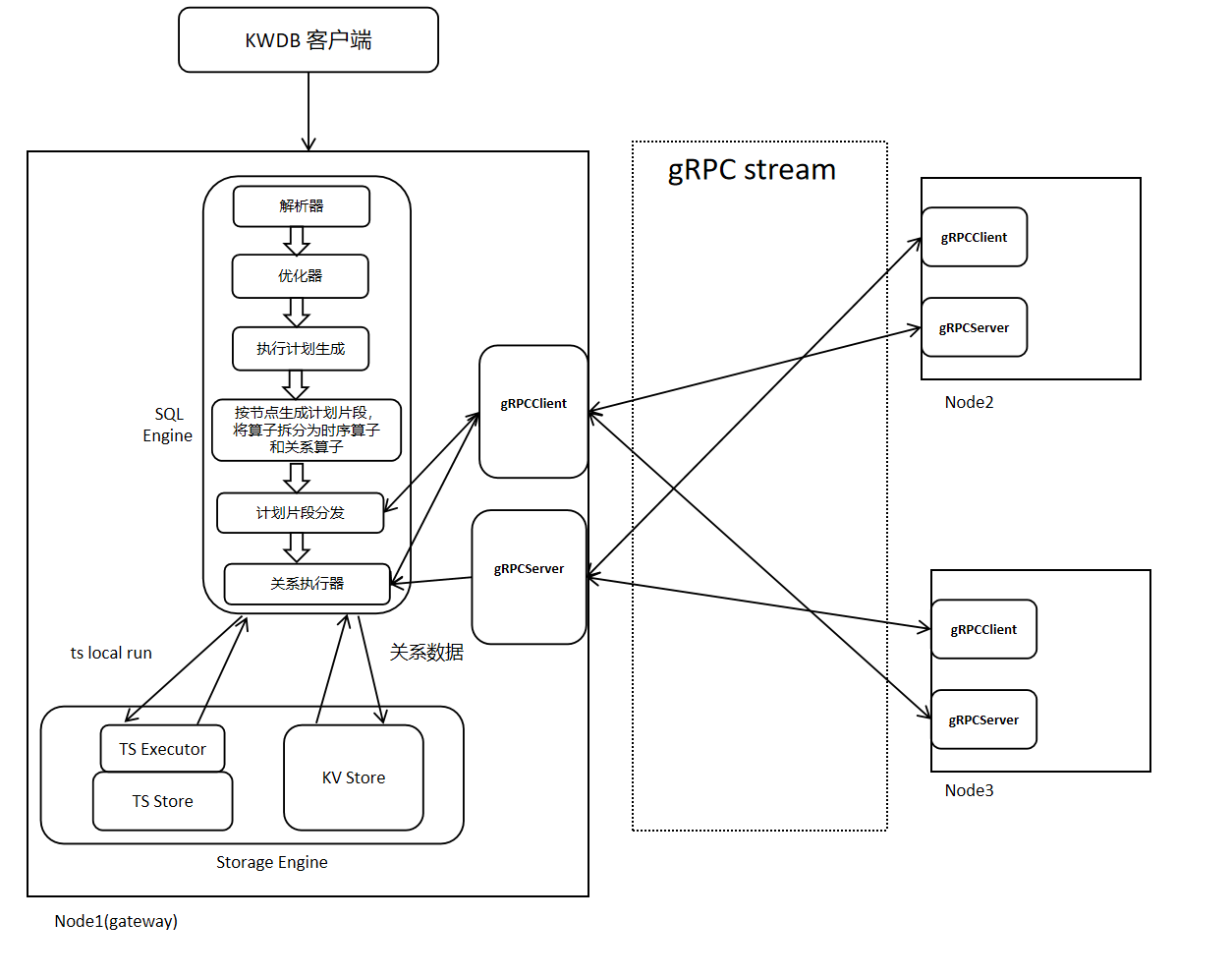
KWDB's distributed execution architecture is shown in the figure below. Distributed execution relies on distributed physical plans generated during the planning phase, uses gRPC for data and information transmission, performs parallel computation on each node, and finally aggregates results at the gateway node.

The execution flow is as follows:

When a client inputs an SQL statement, after passing through KWDB's parser and optimizer, an expression tree with minimum cost is generated. Subsequently, an executable execution plan is generated based on the given expression tree. The operators in the plan are split into relational operators and time-series operators, and different node plan fragments are generated according to nodes. Each node's plan fragments are distributed to the corresponding nodes, and each node starts execution based on the received plan fragments.

2.1 Flow-Based Execution Plan

2.1.1 Basic Concept Explanations

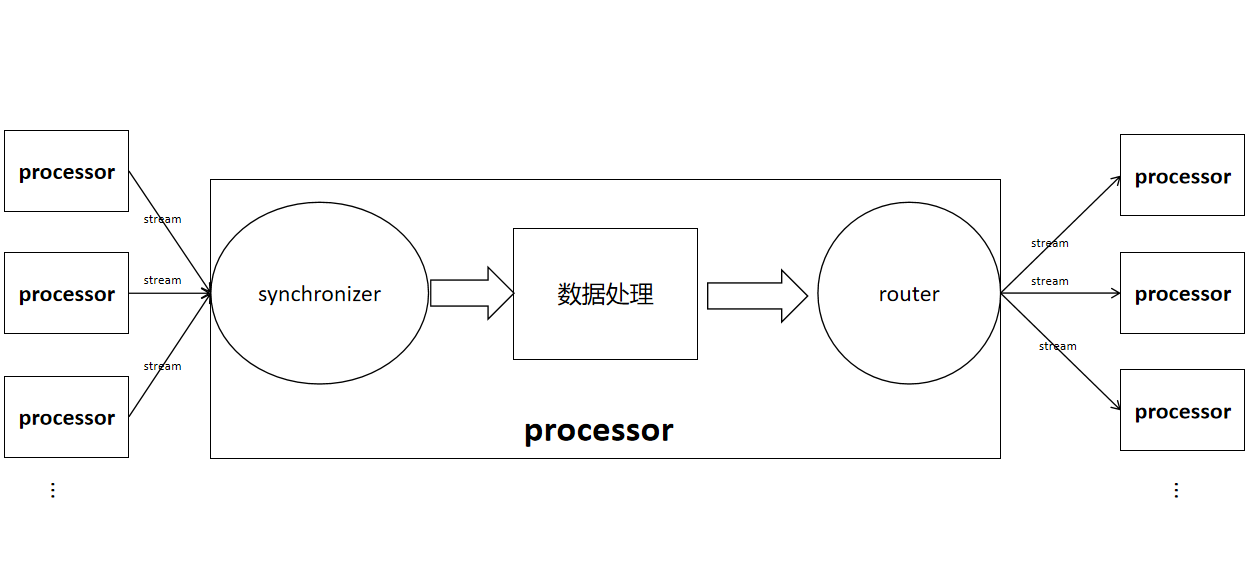
stream: Connects the output router of one operator to the input synchronizer of another operator.

input synchronizer: Used to receive data calculated from child nodes. It is divided into two types based on whether ordering is required: InputSyncSpec_UNORDERED and InputSyncSpec_ORDERED.

router/outbox: Used to send local data to remote operators. An outbox is used when there is only one output stream from an operator, while a router is used when there are multiple output streams. Routers are divided into mirrorRouter, hashRouter, and rangeRouter based on different data transmission methods.

• hashRouter: Hashes certain columns in data rows and selects the node stream to send to based on the hash result.
• mirrorRouter: Replicates table data on each node, sending each row to all output streams.
• rangeRouter: Sends each row to one stream, selecting which stream to send to based on preset boundaries.

The position of streams, synchronizers, and routers in operators, and the connections between operators are roughly shown in the figure below.

FlowSpec: Used to store Flow information. Each node's executor creates that node's Flow based on the received FlowSpec. FlowSpec content includes FlowID (UUID), gateway node id, relational operator information, and time-series operator information.

Flow: Consists of a collection of physical plan nodes, plan node input synchronizers, plan node output routers, and streams. Each node constructs a Flow based on FlowSpec, and the executor performs data calculation and transmission based on the Flow.

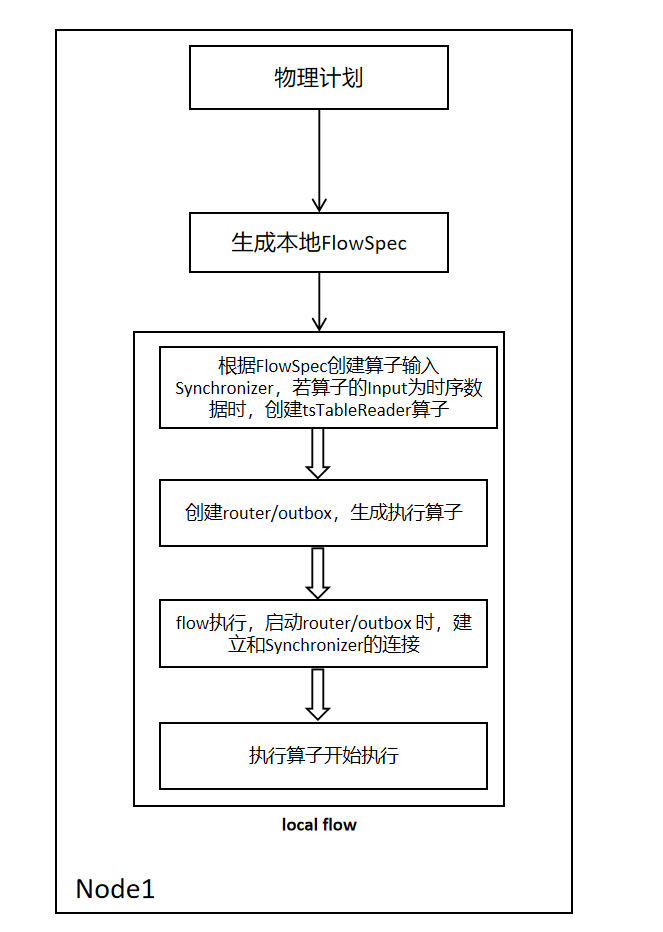
2.1.2 Single Node Flow Setup

The process is as follows single node Flow setup. A local FlowSpec is generated based on the operator information provided by the planning phase. Iterate through the relational operators in FlowSpec, and connect each operator's input and output through channels. When the operator's input is time-series data, a tsTableReader operator is generated and attached to the relational Flow for subsequent time-series Flow creation and data reception.

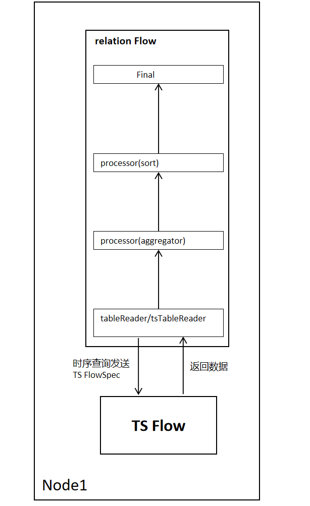
2.1.3 Single Node Flow Execution Process

The single node Flow execution process is as follows. Taking a sort-agg-scan plan as an example, tableReader reads relational data, and tsTableReader reads time-series data. When tableReader/tsTableReader reads each row of data, it returns one row of data to the upper-layer operator until data reading is complete.

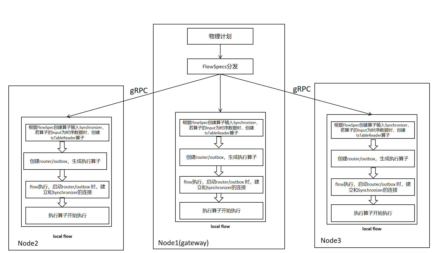
2.1.4 Multi-Node FlowSpec Distribution and Flow Setup

The FlowSpec distribution and Flow setup process are shown in the figure below. Compared with single-node execution, it adds the FlowSpec distribution operation, sending other nodes' FlowSpecs to the corresponding nodes.

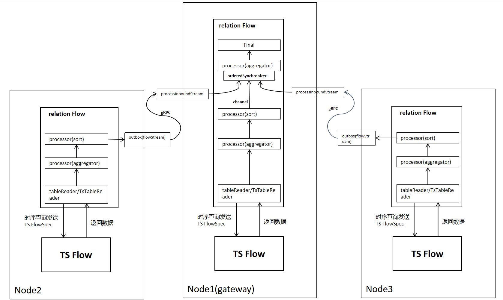
2.1.5 Multi-Node Flow Execution Process

After sending FlowSpec to each node, each node generates the corresponding operator based on the operator specs (Processor/TsProcessor) carried in FlowSpec. Taking a sort-agg-scan plan as an example, data transmission in distributed mode is as follows. Compared with a single node, it needs to add network transmission part, and grouping (group by) aggregation needs to add secondary aggregation.

Cross-node data transmission uses gRPC, while local data transmission uses channels.

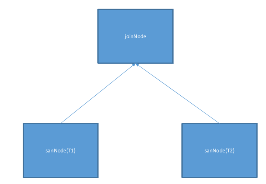
2.1.6 Flow Execution Process When Data Redistribution is Needed (Using Router, Taking OutputRouterSpec_BY_HASH as an Example)

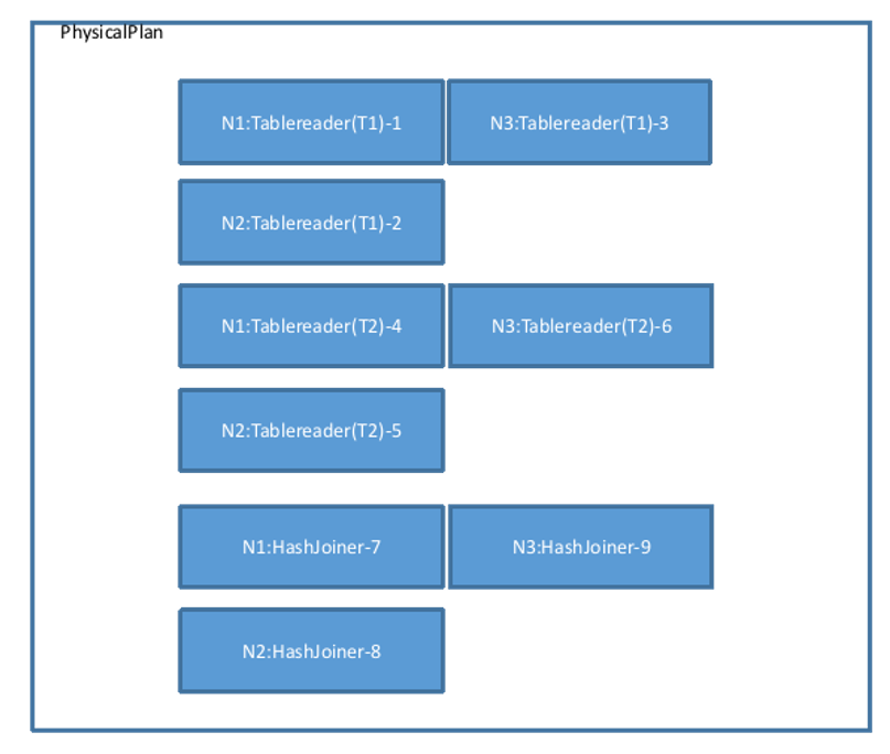
Taking a simple physical plan as an example, this plan represents a Join between two tables T1 and T2. The equality relationship of the Join is T1.k=T2.k. The data of T1 and T2 is distributed across 3 nodes, represented as shown in the figure below:

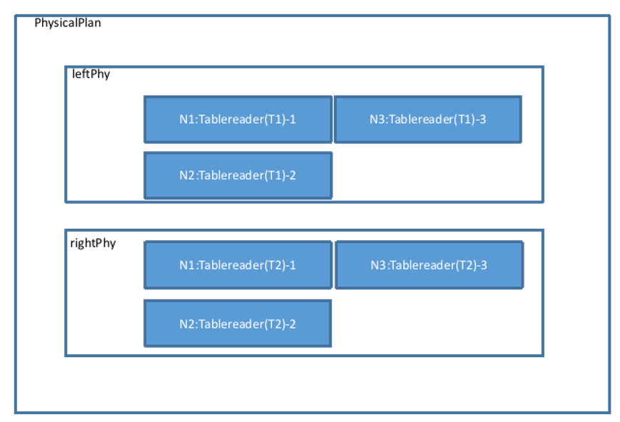
The physical plan confirms data distribution information, sets operations such as Filter and Projection for each Tablereader operator, and finally adds the generated Tablereaders to the physical plan.

Merge the left and right plans:

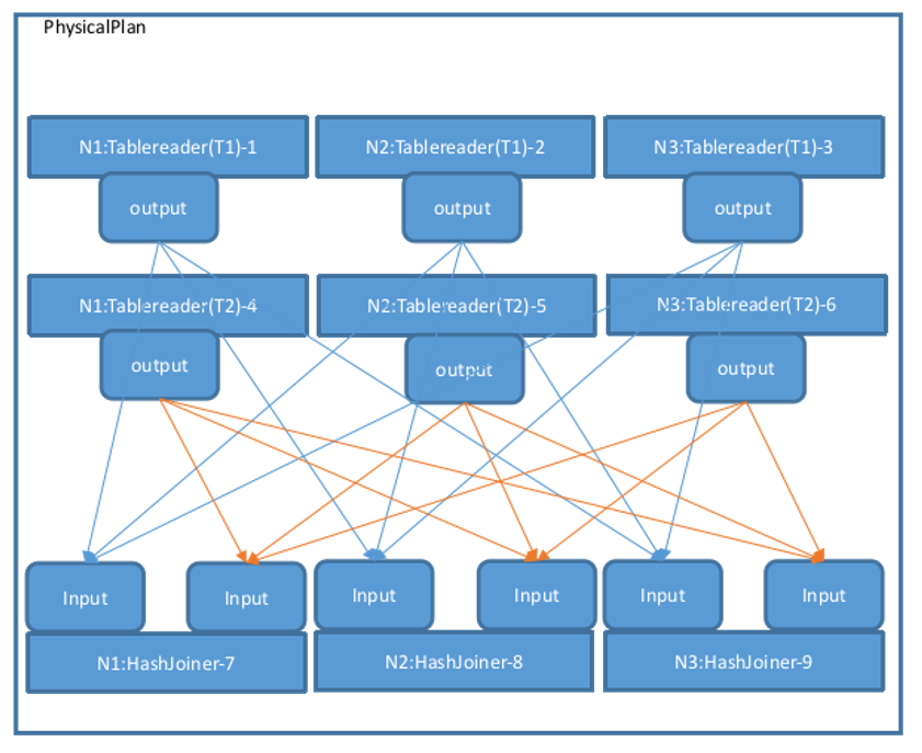
The findJoinProcessorNodes function determines the number of nodes for performing the Join operation. Here, the Tablereader operator is on 3 nodes, so the Join operator will also construct 3 corresponding nodes. Therefore, it calls AddJoinStage to generate 3 HashJoiners (not considering other Join algorithms), and changes the Output type of its left and right operators (here referring to the 6 Tablereaders in the figure) to OutputRouterSpec_BY_HASH (meaning that during execution, cross-node Hash redistribution is required). The physical plan view becomes as shown in the figure below:

Then, call MergeResultStreams to connect the 3 Tablereaders of T1 and T2 to the left and right sides of each HashJoiner according to the number of nodes. Directed arrows represent Streams, starting from one operator's Output and ending at another operator's Input. The physical plan view is as follows. The Output types in the figure are all OutputRouterSpec_BY_HASH:

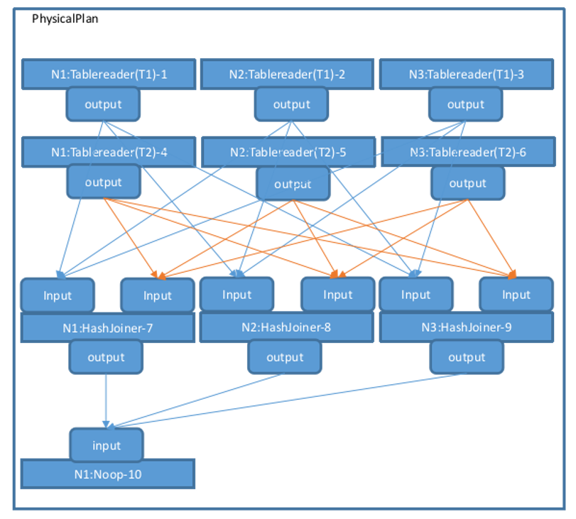
The createPhysPlan function generates the overall topology of the physical plan. The FinalizePlan function adds a Noop operator on top of the existing physical plan to aggregate the final execution results, and then sets the StreamID associated with each operator's Input and Output, as well as the Stream type (StreamEndpointSpec_LOCAL or StreamEndpointSpec_REMOTE). If a Stream connects operators on the same node, it is StreamEndpointSpec_LOCAL; otherwise, it is StreamEndpointSpec_REMOTE. After executing createPhysPlan-->FinalizePlan, the overall physical plan is complete, as shown in the figure below:

During execution, operators are executed in sequence according to this process.

3. Multi-Model Execution Architecture

Database multi-model architecture refers to a database system that can support multiple data models (such as relational, time-series, etc.). Multi-model is the main innovation of KWDB. Its characteristic is that it can achieve cross-model query capability, namely implementing joint queries on different data models. Users can simultaneously retrieve information from multiple data sources, enhancing the depth and breadth of data analysis.

The innovation of multi-model architecture makes the database more efficient and flexible when dealing with diverse data needs, and can better support the development of modern application scenarios. KWDB's multi-model execution architecture supports the following relational operators and time-series operators.

3.1 Relational Execution

3.1.1 Relational Execution Process

Relational execution uses the distributed execution architecture from Chapter 2. Section 3.1.2 adds a detailed introduction to relational operators.

3.1.2 Relational Operators

In a database system, relational operator execution refers to the actual execution of various operators (relational operators) in query statements. Database queries are usually composed of one or more operators, which include selection, projection, join, sorting, etc. They are executed in a specific order and manner to complete query tasks. The following is the general process of relational operator execution:

1. Parse query statements: The database system first parses the query statement, identifies various operators and operands, and constructs a Query Execution Plan.

2. Query optimization: During the construction of the execution plan, the database system performs query optimization, trying to find the most effective execution plan to improve query performance. This may involve selecting appropriate indexes, adjusting join order, reordering operations, and other optimization strategies.

3. Generate execution plan: Once query optimization is complete, the database system generates the final execution plan, which describes the specific steps and order required to execute the query, as well as the relational operators needed for each step.

4. Execute relational operators: Next, the database system gradually executes each relational operator according to the order described in the execution plan. Each relational operator usually processes some input data and generates output for the next relational operator.

5. Return results: Finally, when all relational operators have completed execution, the database system returns the execution results to the user or application.

The following are some common relational operators and their functions:

Relational Operator Name	Relational Operator Function
Sort Operator	Sorts a single result set in ascending or descending order based on one column, outputting a new result set. Its input is a single result set, and output is also a single result set. Sorts one or multiple columns through the Order key sort key.
JoinRead Operator	Performs lookup join between input and the specified index. lookupCols specifies the input columns to be used for index lookup. (joinReader is divided into indexjoin and lookupjoin)
Lookupjoin Operator	For ordinary join algorithms, we note that it is not necessary to perform a full table scan on the inner table for every row of the Outer table. In many cases, the cost of data reading can be reduced through indexes, which is what Lookupjoin is used for. The prerequisite for Lookupjoiner adaptation is that the two tables being joined must have indexes on the corresponding index columns of the Outer table. During execution, it first reads data from the smaller table, then finds the approximate scan range from the index of the larger table, compares the larger table's data with the smaller table's data, and advances the larger table to get the final result.
Indexjoin Operator	IndexJoin performs a join between the secondary index "input" and the primary index "desc" of the same table to retrieve columns not stored in the secondary index. See JoinReader for specific execution details.
Mergejoin Operator	Mergejoin is a join method executed when both left and right joins have indexes.
Hashjoin Operator	Hashjoin is a join method executed when both left and right joins have no indexes.
Zigzagjoin Operator	Works by "zigzagging" back and forth between two indexes and only returning rows with matching primary keys within the specified range.
Window Operator	Window Operator is a processor for executing window function calculations with the same PARTITION BY clause.
RowSourcedProcessor Operator	RowSourcedProcessor is a combination of RowSource and Processor, requiring initialization with its post-processing specification and output row receiver.
Aggregator Operator	Operator function: Groups each row in a single result set based on aggregated columns, performs aggregate function calculations within groups, and outputs the results as new rows.
SampleAggregator Operator	SampleAggregator processor aggregates results from multiple sampler processors and writes statistical data to system.table_statistics.
sampleProcessor Operator	SampleProcessor returns samples (random subsets) of input columns and computes cardinality estimation sketches for column sets. The sampler is configured with sample size and sketch column set. It generates one row of global statistics, one row containing sketch information for each sketch, plus sampled rows up to the sample size.
OrdinalityProcessor Operator	OrdinalityProcessor is the processor for the WITH ORDINALITY operator, which adds an extra ordinal column to results. When a function after the from statement has the WITH ORDINALITY attribute, the returned result set will have an additional integer column starting from 1 and incrementing by 1.
Distinct Operator	Distinct is the physical processor implementation of the Distinct relational operator. Distinct is used to remove duplicate records from query results and return unique different values. Distinct can be used for operations on one or multiple columns. For single column operation, it selects non-duplicate data items from that column; for multi-column operation, it means all columns are non-duplicate, which is equivalent to the entire record after concatenating multiple columns.
SortedDistinct Operator	SortedDistinct is a specialized distinct that can be used when all distinct columns are also sorted.
TableRead Operator	An operator for reading table data. Decodes KV-form data extracted from the storage layer into Row form (rows or tuples) that can be calculated during execution, and performs queries on all physical tables. Its input is a KV dataset. Output is a single result set. The data range queried by TableReader is called Span. A single scan can include multiple Spans, each Span contains a StartKey and an EndKey, and the ranges of multiple Spans cannot overlap.
Noop Operator	Noop operator simply passes rows from the synchronizer to the post-processing stage, used for post-processing stages or final stages of computation that only need the synchronizer to connect streams.

3.2 Time-Series Execution

3.2.1 Time-Series Execution Process

KWDB's time-series engine is a batch computation engine based on the Volcano model, implementing column-oriented batch data computation operations. This engine can efficiently process large-scale data, dividing data into batches according to certain rules. After completing computation on each batch of data, it aggregates it into a batch and returns it. This design fully utilizes the advantages of column-oriented computation while optimizing data transmission and processing efficiency through batch return, greatly improving the performance of the entire system when processing large-scale data.

1. Basic Concepts and Components

1. Operators

   • Scan Operator: Responsible for reading data from the storage engine. Depending on the storage location and distribution of data, it may involve reading data from local disks or obtaining data from distributed nodes over the network. For example, when a query involves a specific table, the scan operator reads table data row by row based on the table's indexes (if any) or full table scan method. If data is stored on multiple nodes, the scan operator obtains data from these nodes in parallel to improve reading speed.
   • Filter Operator: Used to filter data read by the scan operator. According to query conditions, the filter operator checks whether each row of data meets the conditions. If it does, it passes it to the next operator for further processing; otherwise, it discards it. For example, for a query condition "age greater than 18", the filter operator checks whether the age field value in each row is greater than 18. If so, it keeps that row; otherwise, it discards it.
   • Aggregation Operator: Performs aggregate computations on data, such as sum, average, count, etc. The aggregation operator receives data passed from upstream operators and computes data according to the definition of aggregate functions. For example, for a query that needs to calculate the sum of a column in a table, the aggregation operator accumulates the column values of all qualifying data to get the final sum result.
   • Join Operator: Used to merge data from two or more tables based on specified join conditions. The join operator reads data from tables participating in the join according to join type (such as inner join, outer join, etc.) and join conditions, and combines data rows that meet the join conditions into one. For example, when a query needs to join two tables based on a common field, the join operator reads data from both tables separately and matches them based on the field value, merging successfully matched data rows into result rows.

2. Execution Nodes KWDB is a distributed database. Execution nodes in the physical plan represent the physical locations where query operations are actually executed. These execution nodes can be a single database server or a node in a distributed cluster.

   Each execution node is responsible for executing a portion of operations assigned to it in the physical plan. For example, when queries involve large-scale data, the physical plan may assign data scan operations to multiple execution nodes for parallel execution, with each node responsible for scanning a portion of data. Then, these nodes pass scan results to an aggregation node for summary computation.

   Execution nodes communicate over the network to collaboratively complete query tasks in a distributed environment. For example, when a join operation requires cross-node data merging, nodes transmit data over the network, perform partial join operations on their respective nodes, and finally aggregate results to a coordination node.

2. Optimization Strategies

1. Cost-Based Optimization Before generating a physical plan, KWDB evaluates and estimates the costs of multiple possible physical plans. This cost estimation considers multiple factors, including data distribution, execution node performance, network bandwidth, disk I/O speed, etc.

   For example, for a join operation, KWDB considers different join algorithms and join orders, and estimates the execution cost of each option. If both tables being joined have large data volumes and one table has a suitable index, using an index-based join algorithm may reduce costs. Conversely, if both tables have no indexes, a hash-based join algorithm may be more suitable.

   By estimating costs for various possible physical plans, KWDB selects the lowest-cost option as the final physical plan for execution.

2. Data Distribution Awareness Since KWDB is a distributed database with data distributed across different nodes, physical plan generation needs to fully consider data distribution to minimize data transmission over the network.

   For example, when executing a query, if the query condition involves a specific data range and the node location of this data range is known, the physical plan can directly assign the query operation to the node containing that data range for execution, rather than performing a broadcast query across the entire cluster. This greatly reduces network overhead and query execution time.

   Additionally, KWDB dynamically adjusts physical plans based on data distribution. For example, if a node has excessive load or fails, the physical plan can automatically reassign tasks originally assigned to that node to other nodes to ensure normal query execution.

3. Parallel Execution To improve query performance, KWDB fully utilizes the advantages of distributed architecture and supports parallel execution of operations in physical plans.

   For example, for large-scale data scan operations, the physical plan can divide data into multiple chunks and assign them to different execution nodes for simultaneous scanning. Then, scan results from each node are merged and further processed.

   Complex operations such as join and aggregation can also use similar parallel execution strategies. For example, for a join operation between a large table and a small table, the small table can be broadcast to each execution node. Then, each node performs join operations on local large table data and broadcast small table data in parallel, and finally aggregates the results.

3. Execution Process

1. Plan Distribution After generating the physical plan, KWDB's Coordinator distributes the physical plan to each execution node. The Coordinator is responsible for parsing user query requests, generating logical query plans, and converting them into physical plans. Then, according to the operation distribution in the physical plan, the Coordinator sends corresponding operation instructions to each execution node.

   After receiving operation instructions, execution nodes prepare the execution environment according to instructions, including loading required data, allocating memory, initializing operators, etc.

   For example, for a scan operation, the execution node determines the data range and data source to scan according to instructions (such as local disk files or other nodes on the network), and prepares corresponding read operations.

2. Data Processing and Passing Execution nodes execute operators in the order specified in the physical plan. Each operator receives data passed from upstream operators, processes it, and passes the processed result to downstream operators.

   For example, after the scan operator reads data from the data source, it passes data to the filter operator. The filter operator filters data according to query conditions, then passes filtered results to subsequent operators such as aggregation operators or join operators for further processing.

   During data passing, data serialization and deserialization as well as network transmission may be involved. KWDB uses efficient data transmission protocols and serialization technologies to reduce data transmission overhead.

3. Result Aggregation and Return After all execution nodes complete their tasks, they send local computation results back to the Coordinator. The Coordinator is responsible for aggregating and organizing results from each node to get the final query results.

   If query results need to be returned to users, the Coordinator serializes results and sends them to the user client. During result return, the Coordinator also performs some additional processing, such as result set pagination and format conversion, to meet user needs.

   For example, for a paginated query, the Coordinator extracts the corresponding data page from the aggregated result set according to the page number and number of records per page specified by the user and returns it to the user.

3.2.2 Time-Series Operators

3.2.2.1 TSTableReader

The TSTableReader operator is used to read data from data tables.

The TSTableReader operator does not need to consider the four access methods in 3.2. It is isolated through the TSTagReader operator in the design.

Specific functions are as follows:

1. Parse relevant parameters of the physical plan TSTableReader operator.
2. Obtain entity data from the TSTagReader operator.
3. Create storage iterator TsTableIterator by calling storage interface.
4. Read data through TsTableIterator.
5. Data filtering: filter+limit+offset.
6. Return data to the upper-layer operator.

Operator design:

Processors: operator tree

1. Parse Flowspec during initialization to generate operator tree
2. Generate table metadata based on coltypes and colLens

TableMeta: table metadata

TSTableReader: scan operator

1. During Init, parse post spec, generate filter and renders Expr after parsing, initialize scancols.
2. During Start, call TSTagReader operator interface to get entity, call storage interface to generate TsTableIterator.
3. During Next, call storage TsTableIterator->Next interface to generate ResultSet, then perform filter and renders calculation.

Aggregator: agg operator

3.2.2.2 TSTagReader

The TSTagReader operator is used to read data from tag tables. It corresponds to four access methods.

Specific functions are as follows:

1. Parse relevant parameters of the TSTagReader operator in the physical plan.
2. According to accessMode in the plan, call different storage tag access interfaces.
3. Read tag data.
4. Filter tag data through tagfilter.
5. Provide an interface for returning entity data to the TSTableReader operator.

TagIndex/TagIndexTable access method:

Obtain primary tags and scantags information from the plan (can be empty), call storage GetEntityIdList() interface to return entityId list.

KStatus TsTable::GetEntityeIdList(std::vector<void *>primaryTags,
const std::vector<uint32> &TSTableReadertags,
std::vector<EntityIndex> *entityIdList,
ResultSet* res, k_uint32* count);

TagTable access method:

Call storage GetTagIterator interface to create TagIterator.

Call TagIterator::Next to get tag data.

TsMetaData access method:

Temporarily replaced by TagTable access method.

3.2.2.3 Aggregator

Agg operator, consistent with existing relational AGG, supports multi-column expressions and multiple types of Agg.

First, a hash table is built in the operator. Next, tuples are scanned row by row. First, calculate the tuple's hash value and probe the hash table. If the record does not exist, a new record needs to be inserted into the hash table. Conversely, if it exists, execute aggregate functions based on the current tuple and the record found in the hash table, and update the accumulated state in the hash table. Finally, the aggregation result is provided to the upper-layer operator. AVG needs to be converted to SUM and COUNT.

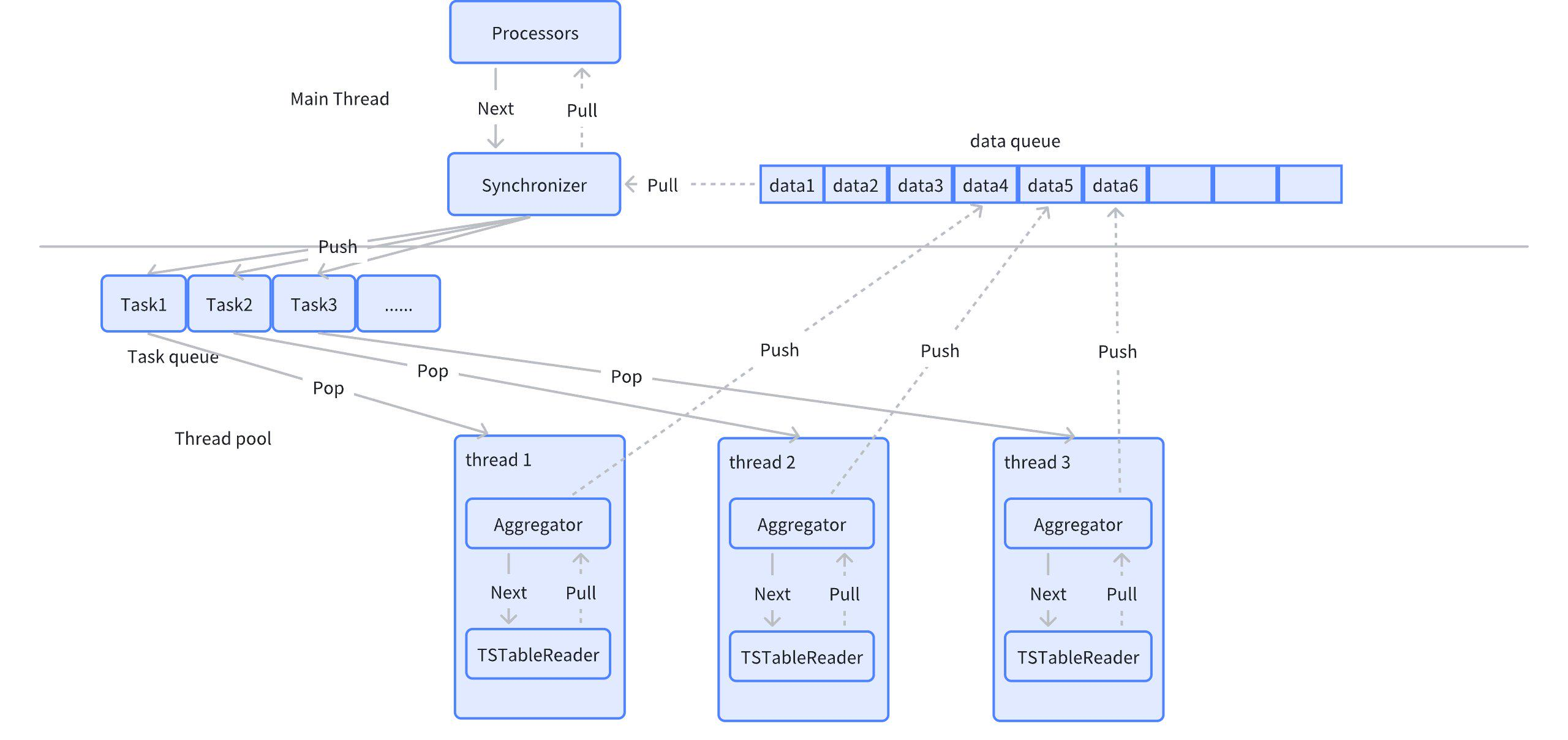
3.2.2.4 Synchronizer

Synchronizer operator, later for ParallelGroup tasks, ParallelGroup can execute in parallel. ParallelGroup can contain Aggregator, Sorter, and at least one TSTableReader. The function of Synchronizer is to gather, accept Push data from concurrent tasks, and return to the upper-layer operator.

The Synchronizer operator serves as a node-level operator, serving as the output of parallel ParallelGroup,承接 multiple ParallelGroup.

3.2.2.5 Sorter

Sorting operator, sorts by given sort columns. Consistent with relational sorter.

4. Cross-Model Execution

Cross-model execution refers to combining the advantages of both time-series data and relational data when processing them to achieve more complex data analysis and queries. Its purpose is to address the following needs:

1. Diversity of Data Types With the development of IoT, financial markets, environmental monitoring, and other fields, time-series data (such as sensor data, stock prices, etc.) and relational data (such as user information, transaction records, etc.) have become increasingly common. Enterprises need to analyze both data types simultaneously to obtain comprehensive business insights.

2. Complex Data Analysis Needs Many application scenarios need to consider both time factors and relationships. For example, when predicting equipment failures, it is necessary to analyze not only the historical operating data of equipment (time-series) but also the relationships and influences between equipment (relational data).

3. Enhanced Decision-Making Capability Through cross-model execution, users can obtain more comprehensive information in a single query, enabling more accurate decision-making. For example, by analyzing customer purchasing behavior (relational data) and consumption trends (time-series data), enterprises can develop more effective marketing strategies.

4. Real-Time Data Processing In many applications, the ability to process time-series and relational data in real-time is crucial. Cross-model execution helps enterprises respond quickly to changes.

5. Data Integration and Management Cross-model execution promotes the integration of different data types, making data management more efficient. Processing multiple data types on a single platform reduces data silos and improves data utilization.

In summary, database cross-model execution meets the needs of modern data analysis for diversified data processing and promotes the development and application of related technologies.

4.1 Cross-Model Execution Support Scenarios

When displaying on the platform, it is necessary to query relational data and time-series data simultaneously to display the required results to users. Currently, to support this scenario, cross-model execution needs to be supported.

For queries involving both time-series tables and relational tables, it is necessary to aggregate time-series table data to the relational side and then perform associated queries and calculations with relational tables.

Specific application scenarios include:

1. Support join queries between relational tables and time-series tables, including inner join, left join, right join, full join.
2. Support nested queries between relational tables and time-series tables, including correlated subqueries, non-correlated subqueries, from subqueries.
3. Support union queries between relational tables and time-series tables, including union, union all, intersect, intersect all, except, except all.
4. Time-series tables include template tables, instance tables, and regular time-series tables.

4.2 Cross-Model Execution Process

Data association computation across different models needs to pull data from different models according to the data source in the query plan. The original architecture supports the coexistence of time-series and relational data in queries. For time-series data, there are targeted pull optimization strategies, such as complex query pushdown, filter pushdown, etc. This requirement plans to relax all usage restrictions on time-series table types on the original basis, only controlling that template tables appear at most once in join associations (template tables involve tag splitting and filtering; if multiple template tables appear, it will increase the difficulty and efficiency of splitting and filtering).

For cross-model execution, only need to assemble the time-series part of the data plan into BoReader operators. During execution, the execution plan pulls time-series part data to the relational side.

To achieve cross-model execution between time-series tables and relational tables (usually including JOIN, UNION, and related and non-related subqueries), the most important thing is to construct different data pull operators for different model data. One is the Scan operator for relational tables, and the other is the TSScan operator for time-series tables.

The relational diagram is as follows:

4.2.1 TsFlow Pushdown Rules

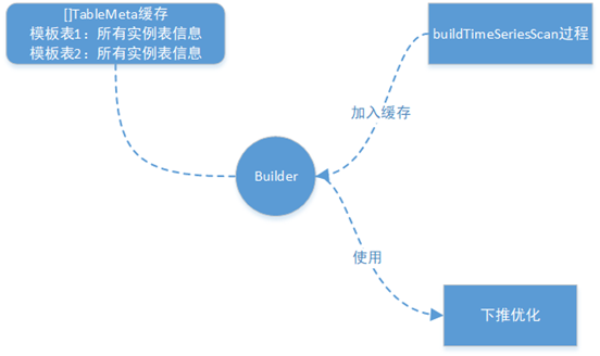
During the TSScanExpr construction phase, template tables require special processing. Obtain all instance table information AllChildInfo (including child table tag values) through the LookUpChildTableInfoBySTbID() interface, and store this information's address in TableMeta for easy expansion of multiple template table scenarios during pushdown optimization.

During the operator construction process triggered by RBO, pushdown rules for TSScanExpr and SelectExpr are added separately. During the TSScanExp construction phase for any time-series table query, a full column query is written and recorded in the TSScanExpr's PushDownSQLArray. Then, during the semantic analysis of other parts of the query statement, if there are filter conditions, it is judged whether the filter conditions can be pushed down. If they can be pushed down, the filter conditions are written into the TSScanExpr's pushdown SQL (through RBO rules, any time-series table query can be pushed down for execution; the worst case is pulling basic columns. This implementation can well satisfy the pushdown of time-series part queries in subquery, join, union, and other cross-model scenarios).

4.2.2 Template Table Pushdown and Expansion

The following figure shows the template table tag column processing and pushdown expansion process. During the template table pushdown optimization phase, respective logical tables are created. During expansion, respective tag column values need to be replaced, and column IDs are referenced according to respective logical tables.

In the multi-template table scenario, during the processing of template tables, each template table's address of all its instance table information is stored in its respective TableMeta. Then, during the above pushdown optimization process, when expanding all template tables, corresponding template table's all child table information is obtained from TableMeta, and then the corresponding tag values are obtained to replace the tags.

4.3 Scenario Use Case Examples

// Relational tables
CREATE DATABASE db;
// All department device management tables
CREATE TABLE db.devices(
owner_id int,  // Department id
device_id int  // Device id
);

// Unit information
CREATE TABLE db.unit_info(
unit_id int,  // Department id
unit_name  varchar(64)  // Department name
);

CREATE TABLE db.device_info(
device_id int,  // Device id
name  varchar(64),// Device name
number varchar(64) // Device number
);

CREATE TABLE db.max_info(
device_id int,  // Device id
electricity double,// Maximum electricity
);

CREATE TS DATABASE tsdb;
// Independent electric meter
CREATE TABLE tsdb.singledevice1(k_timestamp timestamp not null, number varchar(64) not null, electricity double not null) tags (type VARCHAR(64) 'NHB_M1VQ100', serial_number VARCHAR(64) '18120000');

// Template table --- All electric meters
CREATE TABLE device(
k_timestamp timestamp not null,
number varchar(64) not null, // Device number
electricity double not null         // Electricity
) tags (
type VARCHAR(64),        // Electric meter model
serial_number VARCHAR(64) // Box number
);
// Instance table -- Electric meter equipment
CREATE TABLE device_1 USING device (type, serial_number) tags ('NHB_M1VQ2_3','18120407');
CREATE TABLE device_2 USING device (type, serial_number) tags ('NHB_M1VQ2_3','18120407');
CREATE TABLE device_3 USING device (type, serial_number) tags ('NHB_M1VQ2_3','18120407');
CREATE TABLE device_4 USING device (type, serial_number) tags ('NHB_M1VQ2_1','18120405');
CREATE TABLE device_5 USING device (type, serial_number) tags ('NHB_M1VQ2_1','18120405');

// Template table --- All motors
CREATE TABLE machinery(
k_timestamp timestamp not null,
number varchar(64) not null,      // Device number
electricity double not null         // Electricity
) tags (
type VARCHAR(64),        // Motor model
serial_number VARCHAR(64), // Machine number
manufacturer VARCHAR(64)  // Manufacturer
);
1. Join query: Only example given
select unit_info.unit_name, device_info.number, device_info.name, tsdb.device.type, tsdb.device.serial_number,sum(tsdb.device.electricity) from  devices join unit_info on  devices.owner_id = unit_info.unit_id join device_info on devices.device_id = device_info.device_id join tsdb.device on devices.number = tsdb.device.number group by unit_info.unit_name, device_info.number, device_info.name, tsdb.device.type, tsdb.device.serial_number;
2. Nested query: Only example given
select unit_info.unit_name, device_info.number, device_info.name, from  devices join unit_info on  devices.owner_id = unit_info.unit_id join device_info on devices.device_id = device_info.device_id where devices.number in (select number from tsdb.device );
Select electricity > (select max(electricity) from tsdb.device) from db.max_info; // Projection subquery Non-correlated
Select electricity > (select max(electricity) from tsdb.device where electricity < db.max_info.electricity) from db.max_info; // Projection subquery Correlated
Select * from db.max_info where electricity in (select electricity from tsdb.device); // In subquery Non-correlated
Select * from db.max_info where electricity in (select electricity from tsdb.device where number=db.max_info.number); // In subquery Correlated
Select * from db.max_info where exists (select 1 from tsdb.device where electricity=tsdb.t1.electricity); // Exists subquery Correlated
Select * from db.max_info where exists (select 1 from tsdb.device where electricity=db.max_info.electricity and numer in (select numer from db.device_info where db.max_info.device_id=serial_number));// Three-level nesting, Correlated Time-series->Relational->Time-series
Select * from db.max_info where exists (select 1 from tsdb.device where electricity=db.max_info.electricity and numer in  (select numer from tsdb.device_1 where db.max_info.electricity=electricity));// Three-level nesting, Correlated Relational->Time-series->Time-series
select * from (select * from tsb.device where electricity > 100 );
3. Union query: Only example given
Select electricity from db.max_info union select electricity from tsdb.device ;
Select electricity from db.max_info union all select electricity from tsdb.device;
Select electricity from db.max_info intersect select electricity from tsdb.device;
Select electricity from db.max_info intersect all select electricity from tsdb.device;
Select electricity from db.max_info except select electricity from tsdb.device;
Select electricity from db.max_info except all select electricity from tsdb.device;

4.4 Cross-Model Execution Example

Relational table:

Create  table t(a int, b int);

Time-series table:

create table st(e1 timestamp not null,e2 int2 not null,e3 int4 not null)attributes(attr1 bool,attr2 int2, attr3 varchar)
create table c1  using st attributes(true,10,20);
create table c2  using st attributes(false,20,30);

Subquery:

select a in (select e2 from st where e1>'2023-6-16 12:00:00') from t;

As shown in the figure above, the parsing process for the above cross-model execution is: construct ScanExpr for the relational table -> parse query list -> parse subquery.

During subquery parsing, the ConstructTSScan() function creates a TSScanExpr expression for the time-series table. The creation process uses RBO rules to write a full column query. Then, during the semantic analysis of the where clause, ConstructSelect() determines that the condition e1>'2023-6-16 12:00:00' can be pushed down according to rules and updates TSScanExpr. Finally, ConstructProject() eliminates unused columns according to rules and updates TSScanExpr. After pushdown optimization, the template table is expanded into all instance tables' UNION ALL query.

The final plan is:

5. Summary

KWDB, as a distributed multi-model database designed for AIoT scenarios, emphasizes efficiency and flexibility in its design philosophy. As mentioned in the overview, KWDB supports establishing both time-series and relational databases simultaneously and processes multi-model data in a fused manner, providing strong support for applications in the rapidly developing IoT environment.

In this issue's content, we deeply explored KWDB's SQL executor. As an important component of the SQL engine, the executor's design aims to fully leverage KWDB's core advantages, including millions of device connections, millions of data writes per second, and billions of data reads per second. Through efficient execution strategies, KWDB's executor can quickly respond to query requests in rapidly changing data environments, ensuring efficient and stable data processing.

The executor's optimization is reflected not only in its processing speed but also in its high availability and easy operation and maintenance. Through intelligent scheduling and resource management, KWDB can effectively reduce system burden during fused processing of multi-model data and improve overall performance. Additionally, the executor has adaptive capabilities, enabling it to adjust resource allocation based on real-time load, ensuring excellent service quality even during peak periods.

Looking forward, KWDB plans to further enhance the executor's intelligence by adding more machine learning-based optimization algorithms to continuously improve query performance and data processing capabilities. At the same time, the team will focus on expanding the executor's functionality to more flexibly support various complex query and analysis needs, providing users with more comprehensive and efficient data solutions.

In summary, KWDB's SQL executor lays a solid foundation for future development and technological iteration while achieving efficient data processing. We look forward to KWDB leading new directions in database technology for AIoT scenarios through continuous optimization and innovation.